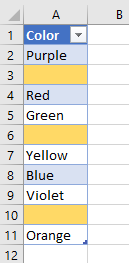
Maybe I’m the odd duck here, but up until recently I ignored the “Conditional Formatting” options in Excel. Boy, was I missing out! Conditional formatting is great, and Excel actually offers some really helpful options. Below, we will walk through highlighting blank cells in Excel, but I encourage you to check out the other possibilities as well.
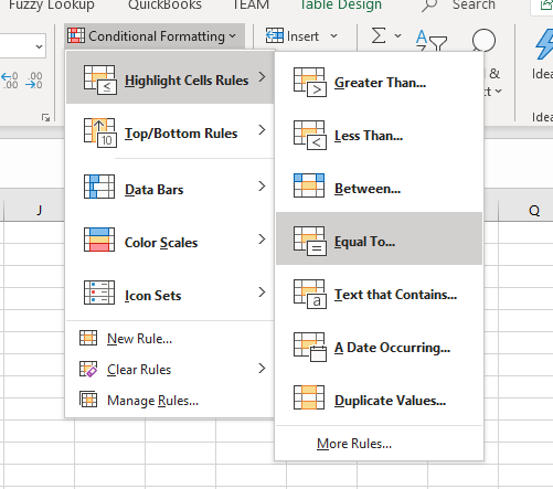
First, make sure your data is formatted as a table. Select the column(s) you want to apply the formatting to, then select the “Conditional formatting” menu item. In this example, we’ll choose “New Rule” below “Icon Sets”:

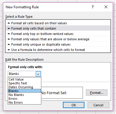
Select “format only cells that contain”, then choose “Blanks” from the “Format only cells with” dropdown. Set the format for the highlighted cells by selecting the “Format” button:


