I recently completed a massive project involving data normalization, and this is the second of two tips that really helped me throughout the process. You may be familiar with VLOOKUP, a function in Excel that allows you to, well, look up values from a separate table. There are some constraints with it, though, for example, you must name a single number to indicate the column that will be returning values. INDEX MATCH combines two functions in Excel and allows you to actually select the column you want to return values from manually with your mouse. To use INDEX MATCH, keep reading!
Just a note– the below article was an incredibly helpful resource when I was learning how to use INDEX MATCH. Please check it out if you want to see additional examples!:
http://www.mbaexcel.com/excel/why-index-match-is-better-than-vlookup/
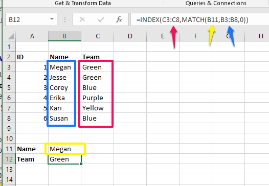
An example of the INDEX MATCH function looks like this:
=INDEX(C3:C8,MATCH(B11,B3:B8,0))

Another way to look at this function is:
=INDEX([Return Values from this list],MATCH([Enter Data in this Cell],[List of Values to Match with Cell Value])
I used this function to match serial numbers from two different tables, to return the unit price from one table into another, and it worked flawlessly. I highly recommend experimenting with this function! It’s a great one.

